on April 27, 2022

Game of life

Conway’s Life is an example of zero-player game, whose evolution is determined by the initial state.

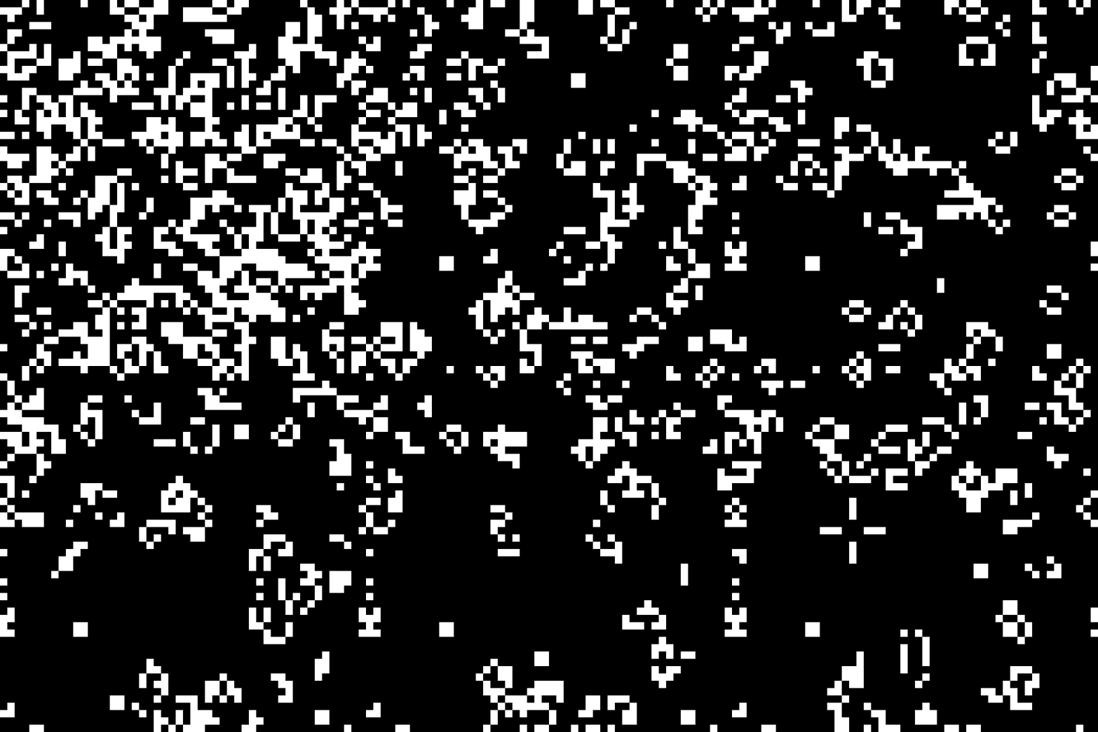
The game happens on a two-dimensional Cellular Automaton with a simple local update rule that can produce complex global behavior. In a Life configuration, cells in an $n × m$ grid can be either alive or dead (represented by $1$ or $0$ respectively). The life To determine the state of a given cell on the next step, Life considers the $3 × 3$ grid of neighbors around the cell. Every step, cells with exactly two alive neighbors will maintain their state, cells with exactly three alive neighbors will become alive, and cells with any other number of neighbors will die. Despite the simplicity of the update rule, Life can produce complex output over time.

demo

Each update is known as a generation.

Different types of patterns occur in the Game of Life, classified by their behaviour. Three different types of patterns are:

Still life does not change from one generation to the next.

demo

Oscillator returns to initial state after a finite number of generations.

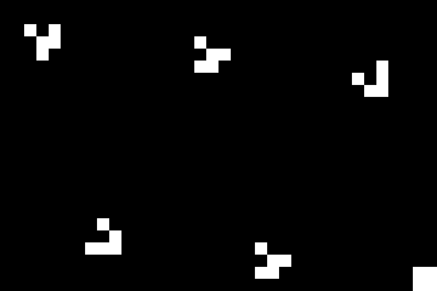
demo Spaceship translate themselves across the grid.

demo

Code for GoL


N=50
T = 100

def update(A):
    A_new = A.copy()
    for m in range(1,A.shape[0]):
        for n in range(1,A.shape[1]):
            i =A[m,n]
            sum_neighbours=sum( [A[m,(n-1)%N],A[m,(n+1)%N],A[(m-1)%N,n],A[(m+1)%N,n],A[(m+1)%N,(n+1)%N],\
                                 A[(m-1)%N,(n-1)%N],A[(m+1)%N,(n-1)%N],A[(m-1)%N,(n+1)%N]])
            if i==1:
                #cell is alive
                if sum_neighbours ==2 or sum_neighbours ==3:
                    A_new[m,n] = 1
                else:
                    #over or under population
                    A_new[m,n] = 0
            if i==0:
                if sum_neighbours==3:
                    A_new[m,n] = 1
                else:
                    A_new[m,n] = 0
    A = A_new
    return A


A = np.random.choice([0, 1], size=((N)*(N),), p=[0.7, 0.3]).reshape((N),(N))
    
for niter in range(100):
    A = update(A)
    fig, ax = plt.subplots(figsize=(10,10))
    im = ax.imshow(A,cmap="gray")
    ax.axis("off")
    plt.show()

← → Top