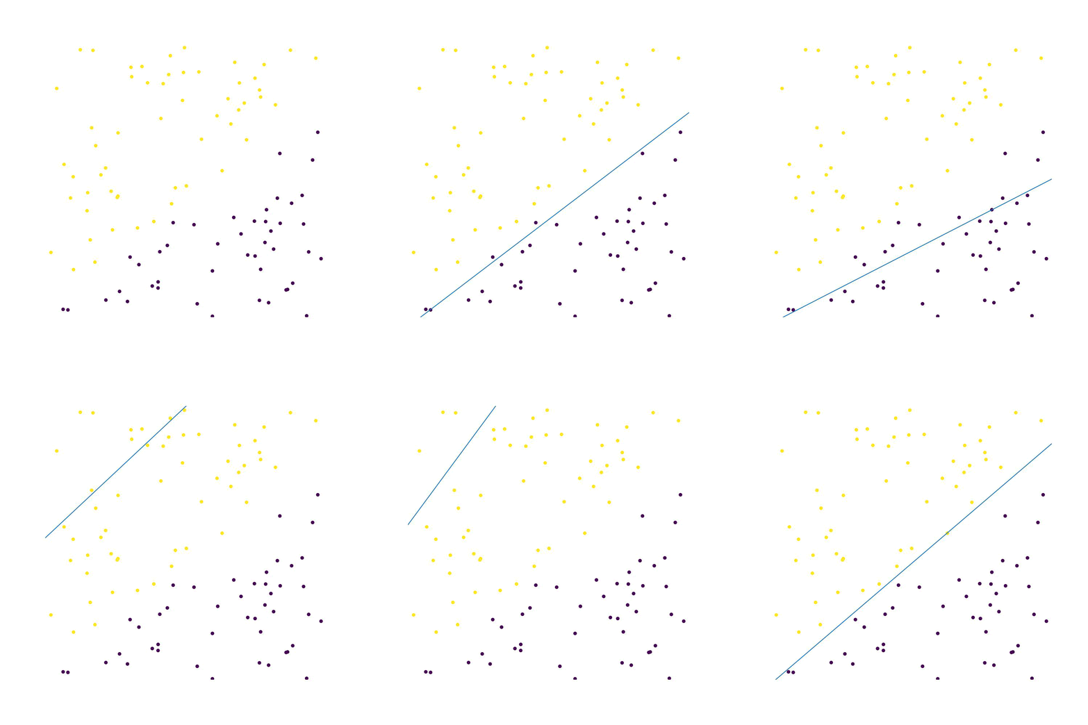
on
Perceptron
Perceptron is a type of artificial neural network. The perceptron is as good as a Classification algorithm. The perceptron works by finding a hyperplane that separates points with different labels in the training set, as long as they are linearly separable.
Consider a function $g(\textbf{x})\rightarrow {0,1}$ which is what we want to approximate. If the function is parameterised by a set of coefficients ${w_1,w_2, …,w_n}=\textbf{w}$, then the function can be rewritten in the form of an inner product $\textbf{w} \cdot \textbf{x}$ . We further add bias term $b$, which leads to a function which is a binary classifier: $f(\textbf{x}) = \begin{cases}1 \text{ if } \textbf{w}\cdot \textbf{x}+b > 0 \ 0 \text{ otherwise.}\end{cases}$ (1) Essentially, we aim to find a line which separates the two categories. Points that fall above the line are of category “high” - $+1$, and all else are of “low” category - $-1$. $b$ is a value which is independent of the input values and allows for inference which is independent from the point of origin: observe that in eq. (1) we are trying to classify points as falling above or below $(0,0…,0)$, which is our origin.
Pseudoalgorithm:
- Initialise the weights to either $(0,0,…,0)$ or a random value: $\textbf{w} = \textbf{w}_0$ .
- Collect a set $\left[(\textbf{x}^{(1)},l_1),(\textbf{x}^{(2)},l_2),… ,(\textbf{x}^{(s)},l_s)\right]$ of $s$ training samples where $\textbf{x}^{(i)}\subset \mathbb{R}^n \quad\forall i$, we use index $m$ to denote a coordinate in an $n$-dimensional space that relates to features of each point, and $l_i\in {0,1}$ is a category of the $i$th object.
- while cost function $C(\textbf{w}(t))=\frac{1}{2}\sum_{i=1}^{n}\left(l_i- f\left(\textbf{w}(t)\cdot \textbf{x}^{(i)} +b\right) \right)^2$ is larger than predefined value:
- for each $i\in s$:
- compute $f\left(\textbf{w}(t) \cdot \textbf{x}^{(i)} +b\right)=f\left(\sum_{m=1}^n w_m(t) x_{m}^{(i)} + w_0(t)\cdot 1\right)= \hat{y}_i$ .
- Compute an update for the weight $m$ wrt sample $i$ $$\Delta w_m^{(i)}(t)=\eta (l_i-\hat{y}i)x{m}^{(i)}$$ (2). The right term means the following: since there’s a discrepancy between the true label and the expected label, the weight has to change. It has to decrease if $l_i<\hat{y}_i$ ( assuming $x$ is always positive), since the label was over-estimated. One can do this for all labels at once: $\Delta \textbf{w}^{(i)}(t)=\eta (l_i-$, $\hat{y}_i)$ , $\textbf{x}^{(i)}$ .
- Update the weights $\textbf{w}(t+1)=\textbf{w}(t)+\Delta\textbf{w}^{(i)}(t)$.
- for each $i\in s$:
- (If offline learning) Update weights $\textbf{w}(t+1) = \sum_{i}\Delta \textbf{w}^{(i)}(t)+\textbf{w}(t)$
- Return to step 3, and iterate until convergence.


### Perceptron

"""
import numpy as np
import matplotlib.pyplot as plt
from PIL import Image

import os
import glob
images = []


class Perceptron:

    def __init__(self, X, y):
        # shape: arr: (sample,features), labels: (sample,)

        self.n_samples = X.shape[0]
        self.n_features = X.shape[1]
        self.y = np.array(y)
        self.weights = np.random.random(size=self.n_features + 1)/100 #add bias term
        self.learning_rate = 0.05
        X = np.concatenate([X, np.ones((self.n_samples, 1))], axis=1) #
        self.X = np.array(X)


    def fit(self,n_iter=1):

        fig, ax = plt.subplots(figsize=(10,10))
        ax.scatter(self.X[:,0],self.X[:,1],c = self.y)
        x2 = np.linspace(0,1,100)
        x1 = -(x2*self.weights[0] +self.weights[2])/self.weights[1]
        ax.plot(x2,x1)
        ax.axis("off")
        ax.set_title("iteration: 0")
        ax.set_ylim(0,1)
        ax.set_xlim(0,1)
        plt.savefig(f"figures/perceptron_learning_0.jpg", dpi=100)
        pil_im = Image.open(f"figures/perceptron_learning_0.jpg","r")
        # plt.close(fig)

        for niter in range(n_iter):
            for i in range(self.n_samples)[:]:
                x = self.X[i]
                yhat = f(self.weights, x)
                self.weights = self.weights + self.learning_rate * (self.y[i] - yhat) * x
                #

                if niter % 2==0 and (i %10 == 0 or niter == 0):
                    fig, ax = plt.subplots(figsize=(10,10))
                    ax.scatter(self.X[:,0],self.X[:,1],c = self.y)
                    x2 = np.linspace(0,1,100)
                    x1 = -(x2*self.weights[0] +self.weights[2])/self.weights[1]
                    ax.plot(x2,x1)
                    ax.axis("off")
                    # ax.set_title("iteration: "+ str(niter))
                    ax.set_ylim(0,1)
                    ax.set_xlim(0,1)
                    id= np.random.rand()
                    plt.savefig(f"figures/perceptron_learning_{niter}_{id}.jpg", dpi=100)
                    pil_im = Image.open(f"figures/perceptron_learning_{niter}_{id}.jpg","r")
                    # plt.close(fig)
                    # plt.show()
                    images.append(pil_im)

            print(self.cost_function())
            if self.cost_function() <0.05:
                break

    def cost_function(self):
        return sum([(self.y[i] - f(self.weights, self.X[i]))**2 for i in range(self.n_samples)])/2

    def predict(self,Z):

        Z = np.concatenate([Z, np.ones((Z.shape[0], 1))], axis=1)
        y= np.array([f(self.weights,Z[i]) for i in range(Z.shape[0])])
        return y


def f(w, x):
    if np.dot(w, x) > 0:
        return 1
    else:
        return 0

def line(w, x):
    return np.dot(w, x)


if __name__ =="__main__":

    my_array = np.random.uniform(size=(100,2),low=0,high=1)
    k=0.8
    b= 0
    my_label = []
    for i in range(my_array.shape[0]):
        if my_array[i][1] > line(np.array([k,b]), np.array([my_array[i][0],1])):
            my_label.append(1)
        else:
            my_label.append(0)

    # plt.scatter(range(100),my_array,c = my_label)
    plt.scatter(my_array[:,0],my_array[:,1],c = my_label)
    plt.title("training set")
    plt.show()


    model = Perceptron(my_array,my_label)
    model.fit(10)

    new_array = np.random.uniform(size=(1000,2),low=0,high=1)
    new_label = []

    for i in range(new_array.shape[0]):
        new_label.append(f(model.weights,np.array([new_array[i][0],new_array[i][1],1])))
    new_label = model.predict(new_array)

    fig, ax = plt.subplots(figsize=(10,5),ncols=2)
    ax[0].scatter(my_array[:,0],my_array[:,1],c = my_label)
    x2 = np.linspace(0,1,100)
    x1 = -(x2*model.weights[0] +model.weights[2])/model.weights[1]
    ax[0].plot(x2,x1)
    ax[0].axis("off")
    ax[0].set_title("train set")

    ax[1].scatter(new_array[:,0],new_array[:,1],c = new_label)
    x2 = np.linspace(0,1,100)
    x1 = -(x2*model.weights[0] +model.weights[2])/model.weights[1]
    ax[1].plot(x2,x1)
    ax[1].axis("off")
    ax[1].set_title("test set")

    plt.savefig("perceptron_training1.jpg", dpi=100)


    images[0].save('perceptron_learning1.gif',
                   save_all=True, append_images=images[1:], duration=15, loop=0)


    files = glob.glob('./figures/*')
    for f in files:
        os.remove(f)