Attractors

The basin of attraction is the set of initial conditions from which the solutions converge asymptotically to a given attractor. Since the basin can include the points quite distant from the attracting set, the size of the basin, as a general rule, is not determined by the local properties of the attractor. . In dissipative maps and flows, it is delimited by the complex geometrical configuration of stable manifolds of unstable invariant sets, which can lead to fractal boundaries[1]

sync basin is the attraction basin of the state of full synchronization for which, in the appropriate corotating reference frame, all oscillators share the steady phase value.

Strange attractors can be the cause of turbulent or chaotic behaviours.

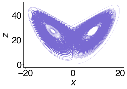
A classical example of a system analysed via attractor lens is a system of three ODEs (the Rosler system): $\dot{x} =-(y+z)$ $\dot{y} =x+0.2y$ $\dot{z}=0.4+xz-5.7z$. This system has a chaotic attractor. Similarly, Lorenz system, described with the following equations

$\dot{x} =-\sigma(y-x)$ $\dot{y} =x(\rho-z)-y$ $\dot{z}=xy-\beta z$. possesses the “butterfly” attractor looked from the x-z plane:

Conjecture For a reconstruction of a $d$-dimensional system, any $d$ independent quantities are sufficient. Any set of $d$ independent quantities which uniquely and smoothly label the states of the attractor are diffeomorphically equivalent.

E.g. instead of looking at $z,y,x$, one can look at $\dot{x},\dot{y},z$ and still be able to reconstruct 3-dimensional dynamics. Even more so, it is possible to reconstruct the dynamics by looking at a set of timesteps of one variable, e.g. $x(t),x(t-\tau),x(t-2\tau)$.

System’s dimension

The “dimension” of a system being observed corresponds to the number of independent quantities needed to specify the state of the system at any given instant. Thus the observed dimension of an attractor is the number of independent quantities needed to specify a point on the attractor. Note that the topological dimension of the attractor is directly related to the number of nonnegative characteristic exponents. A spectrum of all negative characteristic exponents implies a pointlike zero-dimensional attractor; one zero characteristic exponent with all others negative implies a one dimensional attractor; one positive and one zero characteristic exponent corresponds to the observation of folded-sheet-like structures making up the attractor; two positive characteristic exponents correspond to volumelike structures; and so on.

If the phase-space is obtained from values of some variable along with time-delayed values of the same variable, slicing of the space is obtained by forming a conditional PDF: $P(x_t|x_{t-\tau},x_{t-2\tau},…,x_{t-k\tau})$. If we take $\tau$ to be small, the $k$ conditions are equivalent to specification of the value of x at some time along with the value of all its derivatives up to order $k-1$. We need to have $\tau«I/\Gamma$ where is the degree of accuracy with which one can specify a state, and where $\Gamma$
is the sum of all the positive-characteristic exponents. The dimensionality of the attractor is the number of conditions needed to yield an extremely sharp conditional probability distribution, in which case the system is determined by the conditions.

The maximal Lyapunov exponent is obtained with a the procedure that consists of making a cut along the attractor, coordinatizing it with the unit interval (0, 1), and accumulating a return map $x(t)=f(x(t-1))$ by observing where successive passes of the trajectory through the cut occur. $\lambda(x_0)=\lim_{n\rightarrow \infty}\frac{1}{n}\sum_{i=0}^{n-1}\ln|f’(x_i)|=\lim_{n\rightarrow \infty}\frac{1}{n}\ln|D_{x_0}f^t(x_0)u_0|$ . For the whole spectrum of the exponents,consider first a point $x_0$ and an infinitesimal perturbation $u_0$. after time $t$, their images will become $f^t(x_0)$ and $f^t(x_0+u_0)$ and the perturbation becomes $u_t= f^t(x_0+u_0)-f^t(x_0)= D_{x_0}f^t(x_0)u_0$. with a linear approximation. Therefore the average exponential rate of divergence is as defined above.

from scipy.integrate import odeint
import numpy as np

def derivative(vec,t, dynamics = "Rossler"):
    if dynamics == "Rossler":
        x,y,z= vec
        dxdt = -(y+z)
        dydt = x + 0.2*y
        dzdt = 0.4 + x*z - 5.7*z
    if dynamics == "Lorenz":
        beta = 8/3
        rho = 28
        sigma =10
        x,y,z= vec
        dxdt = sigma*(y-x)
        dydt = x*(rho-z) -y
        dzdt = x*y - beta*z
    return np.array([dxdt,dydt,dzdt])



dt=0.01
T=500
t = np.linspace(0, T, int(T/dt))
timeseries = odeint(derivative, np.array([1,1,0]), t, args = ("Lorenz",))

plt.plot(timeseries[:,0],timeseries[:,2],linewidth=0.3,alpha=0.9,color= "slateblue")
plt.xlabel("$x$")
plt.ylabel("$z$")
plt.show()

References

[1] E. Ott, Chaos in Dynamical Systems (Cambridge University Press, Cambridge, UK, 2002).

[2] Geometry from a Time Series N. H. Packard, J.P.Crutchfield, J.D.Farmer, and R.S.Shaw (PRE, 1979)